


Abstract
The Sustainable Development Goals target to achieve Universal Health Coverage (UHC), including financial risk protection (FRP) among other dimensions. There are four indicators of FRP, namely incidence of catastrophic health expenditure (CHE), mean positive catastrophic overshoot, incidence of impoverishment and increase in the depth of poverty occur for high out-of-pocket (OOP) healthcare spending. OOP spending is the major payment strategy for healthcare in most low-and-middle-income countries, such as Bangladesh. Large and unpredictable health payments can expose households to substantial financial risk and, at their most extreme, can result in poverty. The aim of this study was to estimate the impact of OOP spending on CHE and poverty, i.e. status of FRP for UHC in Bangladesh. A nationally representative Household Income and Expenditure Survey 2010 was used to determine household consumption expenditure and health-related spending in the last 30 days. Mean CHE headcount and its concentration indices (CI) were calculated. The propensity of facing CHE for households was predicted by demographic and socioeconomic characteristics. The poverty headcount was estimated using ‘total household consumption expenditure’ and such expenditure without OOP payments for health in comparison with the poverty-line measured by cost of basic need. In absolute values, a pro-rich distribution of OOP payment for healthcare was found in urban and rural Bangladesh. At the 10%-threshold level, in total 14.2% of households faced CHE with 1.9% overshoot. 16.5% of the poorest and 9.2% of the richest households faced CHE. An overall pro-poor distribution was found for CHE (CI = −0.064) in both urban and rural households, while the former had higher CHE incidences. The poverty headcount increased by 3.5% (5.1 million individuals) due to OOP payments. Reliance on OOP payments for healthcare in Bangladesh should be reduced for poverty alleviation in urban and rural Bangladesh in order to secure FRP for UHC.
Introduction
Key Messages
CHE incurred by 14.2% of households nationally.
CHE was more concentrated into rural (16.3%) than urban (8.6%) population and towards the households with lower socioeconomic status.
3.5% of total population fell into poverty annually due to OOP spending for healthcare, which corresponds to economic impoverishment of 5 million people in Bangladesh.
In recent years, a large literature on OOP payments and its impact on CHE and poverty has been developed (Wagstaff and van Doorslaer 2003; Xu et al. 2003; van Doorslaer et al. 2006, 2007; Amaya Lara and Ruiz Gómez 2011; Chuma and Maina 2012; Tomini et al. 2012). From a study of 89 countries, incidence of CHE was estimated to 3.1, 1.8 and 0.6% in low-, middle- and high-income countries, respectively (Xu et al. 2007). The incidence of CHE in households of Bogota in Colombia was 4.9% and this incidence was higher in low-income households without any affiliation to social security schemes (Amaya Lara and Ruiz Gómez 2011). Flores et al. (2008) estimated CHE for inpatient care in India to 30%. Chuma and Maina (2012) observed that ∼1.48 million Kenyans were pushed below the national poverty line due to OOP payments and the burden was found to be highest among the poor (Chuma and Maina 2012). In Burkina Faso, ∼6–15% of households experienced CHE when using 40% of total non-food expenditure as a threshold. Household economic status was a key determinants of CHE along with household health care utilization type, illness episodes and presence of chronic illness (Su et al. 2006). In Uganda, 2.9% of households incurred CHE in 2003 (Xu et al. 2006). In Nigeria, 40.2% of households faced CHE when using a 10% threshold level of total expenditure. This estimate was lower, 14.8%, when a 40% threshold level was used (Onoka et al. 2011). In a multi-country analysis, van Doorslaer et al. (2006) observed that in 11 Asian countries 2.7% of the population under study (78 million people) fall below the poverty-line due to OOP payments for healthcare (van Doorslaer et al. 2006). In another multi-country study, Bangladesh appeared as the most affected country with the highest incidence (15.6%) of CHE (Van Doorslaer et al. 2007).
Two studies have been published in recent years which have analysed the impact of OOP payments for healthcare on economic impoverishment and poverty in Bangladesh (Rahman et al. 2013; Hamid et al. 2014). Rahman et al. (2013) using data from a metropolitan city (Rajshahi) of Bangladesh investigated the determinants of high healthcare expenditure and healthcare-related financial catastrophe. This study found that the households spent on average 11% of their budget on health. Half of the residents spent 7% of the monthly per capita consumption expenditure for one illness and ∼9% of all households faced financial catastrophe. The socioeconomic pattern of health expenditure showed that though the poorest households spent less on health, they faced financial catastrophe more than four times than the richest households. It was also observed that the risk of financial catastrophe and the level of OOP payments were higher in relation to inpatient and outpatient care from both public and private facilities, compared with self-medication and care from traditional healers. The analysis suggests that socioeconomic status, presence of chronic and childhood and adult illness appeared as the determinants of OOP payments. Hamid et al. (2014) employed data from rural households of 14 districts (out of 64) which were members of a social business company, named Grameen Kalyan, which had been operating a pre-paid card based micro health insurance scheme. This study investigated the impact of OOP payments for healthcare on people falling into poverty overall as well as in relation to particular diseases. It found that 3.4% of households annually fell into poverty due OOP spending for healthcare and that non-communicable diseases were the principal reason for the effect. While both studies contribute to the knowledge base of the impact of OOP healthcare spending on economic impoverishment in Bangladesh, both reflect a partial picture of the country. Rahman et al. (2013) investigated the issue in a metropolitan city and focused on catastrophe related to OOP spending. It consequently missed the catastrophe in rural areas and also poverty impact in both urban and rural areas separately. Hamid et al. (2014), on the contrary, missed the catastrophic impact estimation in total population and poverty impact in urban population. That study included only the low-income population, who were members of a rural micro-insurance scheme and as a result missed the general economic structure of the country, which is important while studying poverty. It is important to study the impact of OOP healthcare spending on economic impoverishment/poverty reflecting the national situation as well as the urban and rural scenarios.
In this study, the authors investigated the impact of OOP payments on CHE and poverty in Bangladesh using the latest national Household Income and Expenditure Survey (BBS 2011). The status of FRP for Universal Health Coverage was estimated for Bangladesh. This in-depth analysis may be useful for developing specific policy actions for poverty alleviation related to healthcare financing mechanisms in Bangladesh.
Methods
Data sources
Data were obtained from the latest Household Income and Expenditure Survey 2010 (HIES) of Bangladesh (BBS 2011). HIES is periodically conducted in each 5 years by Bangladesh Bureau of Statistics. This nationally representative survey provides information on all kind of income and consumption of households, including healthcare expenditure. This current survey employed a two-stage stratified random sampling technique and a total sample of 12 240 households were selected. In the first stage, 1000 primary sampling units (PSUs) from 16 strata (6 rural, 6 urban and 4 SMAs) across the country were selected. Each PSU consists of 200 households. In the second stage, 20 households were randomly selected from each PSU (BBS 2011). All analyses in this study were conducted using STATA-13.0. Since two-stage stratified random sampling method was employed for data collection, the analyses accounted for probability sample weight.
Measuring incidence and intensity of CHE
The incidence of CHE was estimated from the fraction of OOP payments for healthcare in relation with household consumption expenditure, which exceeds a certain threshold (Wagstaff and van Doorslaer 2003). Two definitions are often used for such estimations. Firstly, OOP expenditure is compared with total household consumption expenditure (THCE) (Pradhan and Prescott 2002; Wagstaff and van Doorslaer 2003; Russell 2004) and secondly, such expenditure is compared with the total non-food consumption expenditure (NFE) of households (Berki 1986; Xu et al. 2003, 2006). OOP healthcare expenses of all individuals in a household are summed up and compared with the same household’s consumption expenditure for assessing if the household faced CHE at different levels of thresholds. There is no single accepted threshold for estimating CHE. However, households that incur 10% of THCE and 25% of NFE have been used as the CHE thresholds in this study. For observing sensitivity, we have applied more threshold levels (5 and 15% of THCE and 15 and 40% of NFE). While applying the first threshold for CHE is generally recommended at 10% level and corresponding recommended threshold for the second definition lies at 40% level (Wagstaff and van Doorslaer 2003). The CHE incidence measure does not reflect the amount by which households exceed the threshold. The CHE overshoot is thus estimated, which presents by what percentage the households, incurred CHE, and exceeds the threshold.
Asset quintiles and concentration index
Information on land, durable goods, livestock, housing materials and access to basic facilities such as water and sanitation were used for constructing asset index by employing data from HIES (BBS 2011). Categorical asset variables were recorded as binary variables. Principle Component Analysis (PCA) was used to determine the linear weighted combination for asset variables (Vyas and Kumaranayake 2006). The first principal component was used as an indicator of socioeconomic status (O’Donnell et al. 2008). The score associated with the first principal component was divided into five quintiles, which were used as indicators of socioeconomic condition of households in this study. Such socioeconomic categorization had been used in earlier studies (Filmer and Pritchett 2001; Gwatkin et al. 2005). In PCA, frequency weights of number of household members were used for adjusting the effect of household size on asset (Deaton and Paxson 1998).
The concentration indices (CI) were estimated to show the magnitude and direction of the incidence and intensity of CHE across socioeconomic groups of households. In calculating CI, households were ranked according to their socioeconomic condition (asset score), starting with the least wealthy ones. CI was earlier estimated from micro data with a categorical welfare variable or grouped data, which was followed in this study (Kakwani et al. 1997).
Prediction model of CHE
In multilevel logistic regression model we predicted the likelihood of facing CHE by households with explanatory variables containing the information about demographic and socioeconomic level. We used this analysis to account for the hierarchical structure of two level of data, namely, location (urban or rural) and household (Subramanian et al. 2003). From this analysis, we estimated to what extent different explanatory variables influenced the household’s probability for facing CHE. Dependent variable was constructed as a dichotomous variable where 0 and 1 denote the households that facing and not facing CHE, respectively. Models 1 and 2 used total household consumption expenditure and NFE based thresholds for estimating CHE.
Estimating poverty
The poverty headcount was estimated using ‘total household consumption expenditure and such expenditure without OOP payments for healthcare separately. The difference between these two poverty headcount measurements captured the impact of OOP payments on poverty. The national level estimates for poverty line provided by Bangladesh Bureau of Statistics were employed in this study. The poverty line was estimated using Costs of Basic Need (CBN) approach, which implies that, poverty line represents the level of per capita expenditure at which the members of a household can be expected to meet their basic needs (comprised of food and non-food consumption items). Market price for 11 food items for meeting basic need (rice, wheat, pulses, milk, oil, meat, fish, potato, other vegetables, sugar and fruits) for getting 2122 kcal/day per person was captured for estimating food poverty line (BBS 2011). Then the non-food allowance for poverty line was estimated as the median amount spent for non-food items by the group of households which have per capita food expenditure close to food-poverty line. Finally, the poverty line was the sum of food poverty line and non-food allowances for each geographical region. Our approach for estimating poverty impact of OOP health expenditure was that we first kept OOP health expenditure with consumption expenditure and then removed (OOP expenses) from consumption expenditure for observing what proportion of individuals go below the poverty line.
Results
OOP payments
Table 1 shows the average household OOP spending on healthcare for 30 days, which accounted for 644.6 BDT. OOP healthcare spending of rural households (709.1 BDT) for their illness was significantly higher than that of the urban households (468.5 BDT). However, those who were in socioeconomically better-off positions had higher spending in both urban (CI = 0.044) and rural (CI = 0.198) areas.
The average out of pocket payments in BDT (standard error) per household per month across socioeconomic quintiles and rural urban areas
| Rural | Urban | Total | |
|---|---|---|---|
| Poorest | 421.1 (38.8) | 244.7 (75.4) | 416.7 (37.9) |
| Second | 539.9 (39.0) | 272.5 (41.4) | 518.7 (36.2) |
| Third | 690 (54.0) | 419.9 (85.8) | 648.7 (47.7) |
| Fourth | 872.3 (81.0) | 505.5 (85.9) | 728.2 (60.0) |
| Richest | 2437.8 (768.1) | 491.6 (55.4) | 966.3 (195.4) |
| Total | 709.1 (60.8) | 468.5 (42.2) | 644.6 (45.9) |
| CI | 0.198 | 0.044 | 0.113 |
| SE (CI) | (0.019) | (0.030) | (0.016) |
Incidence and intensity of CHE
Table 2 shows the incidence and intensity of household CHE at 5, 10 and 15% of total expenditure. Incidence and intensity of CHE dropped as the threshold level increased from 5 to 15% of total expenditure in both urban and rural areas and also in all socioeconomic quintiles. We observed a pro-poor incidence of CHE in all threshold levels (5, 10 and 15% of total expenditure) in the urban area. At 5 and 10% threshold level, CHE in rural area was pro-poor. On the contrary, it found to be pro-rich (CI = 0.014) at 15% threshold level. The higher intensity (overshoot) of CHE was observed in the socioeconomically better-off households in the total sample. However, this intensity was in opposite direction in urban and rural areas, being pro-poor and pro-rich in urban and rural areas, respectively. The mean positive overshoot (MPO) shows that on an average, OOP expenditure for all households was 13.7% higher than 10% of total expenditure. At the same threshold level, rural area (13.9%) had a higher MPO than urban (12.8%).
The incidence and intensity of household CHE in different socioeconomic condition of urban and rural areas
| Threshold | Rural | Urban | Total | ||||||
|---|---|---|---|---|---|---|---|---|---|
| 5% | 10% | 15% | 5% | 10% | 15% | 5% | 10% | 15% | |
| Head count (HC) | |||||||||
| Poorest | 29.1% | 16.6% | 10.7% | 19.3% | 10.6% | 6.4% | 28.9% | 16.5% | 10.6% |
| Second | 28.1% | 16.3% | 10.1% | 21.0% | 10.9% | 6.2% | 27.5% | 15.9% | 9.8% |
| Third | 27.7% | 15.9% | 10.0% | 22.0% | 10.2% | 7.5% | 26.8% | 15.0% | 9.6% |
| Fourth | 26.6% | 15.8% | 11.3% | 18.0% | 10.7% | 6.6% | 23.3% | 13.8% | 9.4% |
| Richest | 27.3% | 16.6% | 11.4% | 14.3% | 6.8% | 4.5% | 17.5% | 9.2% | 6.2% |
| Total | 28.0% | 16.3% | 10.5% | 16.7% | 8.6% | 5.5% | 25.0% | 14.2% | 9.2% |
| CI | −0.013 | −0.003 | 0.014 | −0.059 | −0.057 | −0.048 | −0.066 | −0.064 | −0.050 |
| SE(CI) | (0.010) | (0.014) | (0.019) | (0.016) | (0.023) | (0.029) | (0.009) | (0.012) | (0.016) |
| Rich–poor ratio | 0.936 | 0.995 | 1.069 | 0.744 | 0.644 | 0.694 | 0.606 | 0.557 | 0.582 |
| Rich–poor difference | −0.018 | −0.001 | 0.007 | −0.049 | −0.038 | −0.020 | −0.114 | −0.073 | −0.044 |
| Overshoot | |||||||||
| Poorest | 3.3% | 2.2% | 1.5% | 2.1% | 1.3% | 0.8% | 3.3% | 2.2% | 1.5% |
| 2nd | 3.3% | 2.2% | 1.5% | 2.1% | 1.4% | 1.0% | 3.2% | 2.1% | 1.5% |
| 3rd | 3.3% | 2.2% | 1.6% | 2.3% | 1.5% | 1.1% | 3.1% | 2.1% | 1.5% |
| 4th | 3.3% | 2.3% | 1.6% | 2.2% | 1.5% | 1.0% | 2.9% | 2.0% | 1.4% |
| Richest | 3.9% | 2.9% | 2.2% | 1.3% | 0.8% | 0.5% | 1.9% | 1.3% | 0.9% |
| Total overshoot | 3.3% | 2.3% | 1.6% | 1.7% | 1.1% | 0.7% | 2.9% | 1.9% | 1.4% |
| MPO | 11.9% | 13.9% | 15.2% | 10.2% | 12.8% | 13.5% | 11.6% | 13.7% | 14.9% |
| CI | 0.016 | 0.026 | 0.035 | −0.071 | −0.078 | −0.091 | −0.058 | −0.053 | −0.052 |
| SE(CI) | (0.018) | (0.023) | (0.027) | (0.025) | (0.032) | (0.038) | (0.014) | (0.018) | (0.022) |
| Rich–poor ratio | 1.180 | 1.290 | 1.405 | 0.625 | 0.608 | 0.616 | 0.588 | 0.592 | 0.603 |
| Rich–poor difference | 0.006 | 0.006 | 0.006 | −0.008 | −0.005 | −0.003 | −0.013 | −0.009 | −0.006 |
Table 3 showed incidence and intensity of CHE considering threshold in respect to household non-food expenditure with a threshold level of 25%. CHE incidence was 17.5% in the whole sample, but higher incidence was observed in rural (20.7%) than urban (9.0%) areas. CHE overshot was 4.7% in rural and 1.7% in urban areas. We further observed a pro-poor headcount and overshoot of CHE in both urban and rural areas with negative values of the CI. Difference between urban and rural areas was observed considering the size of CI, which implies that CHE headcount and overshot were more pro-poor in urban areas. The MPO was estimated to 22.1% in total sample. The corresponding value was higher in rural (22.6%) than urban (19.2%) areas.
Proportion of household observing CHE on health at different threshold level across asset quintiles
| Threshold | Rural | Urban | Total | ||||||
|---|---|---|---|---|---|---|---|---|---|
| 15% | 25% | 40% | 15% | 25% | 40% | 15% | 25% | 40% | |
| Head count (HC) | |||||||||
| Poorest | 35.8% | 25.6% | 14.7% | 26.0% | 18.3% | 9.8% | 35.5% | 25.4% | 14.5% |
| Second | 31.3% | 20.9% | 11.4% | 26.5% | 16.1% | 8.0% | 30.9% | 20.5% | 11.1% |
| Third | 26.8% | 18.4% | 10.8% | 22.6% | 13.6% | 7.4% | 26.1% | 17.7% | 10.3% |
| Fourth | 24.3% | 16.2% | 8.6% | 17.8% | 11.1% | 6.0% | 21.8% | 14.2% | 7.5% |
| Richest | 22.9% | 14.8% | 8.1% | 10.5% | 5.9% | 2.3% | 13.5% | 8.1% | 3.7% |
| Total | 30.0% | 20.7% | 11.6% | 15.1% | 9.0% | 4.4% | 26.0% | 17.5% | 9.7% |
| CI | −0.080 | −0.092 | −0.098 | −0.156 | −0.184 | −0.198 | −0.149 | −0.173 | −0.189 |
| SE (CI) | (0.010) | (0.012) | (0.017) | (0.017) | (0.22) | (0.032) | (0.008) | (0.011) | (0.015) |
| Rich–poor ratio | 0.640 | 0.579 | 0.555 | 0.404 | 0.321 | 0.234 | 0.381 | 0.317 | 0.256 |
| Rich–poor difference | −0.129 | −0.108 | −0.065 | −0.155 | −0.124 | −0.075 | −0.220 | −0.174 | −0.108 |
| Overshoot | |||||||||
| Poorest | 8.9% | 5.8% | 2.9% | 6.1% | 4.0% | 1.8% | 8.8% | 5.8% | 2.9% |
| Second | 7.4% | 4.8% | 2.4% | 5.3% | 3.2% | 1.5% | 7.2% | 4.7% | 2.3% |
| Third | 6.4% | 4.1% | 2.0% | 4.5% | 2.8% | 1.4% | 6.1% | 3.9% | 1.9% |
| Fourth | 5.4% | 3.4% | 1.6% | 3.8% | 2.4% | 1.1% | 4.8% | 3.0% | 1.4% |
| Richest | 5.3% | 3.5% | 1.7% | 1.7% | 0.9% | 0.3% | 2.6% | 1.5% | 0.7% |
| Total overshoot | 7.2% | 4.7% | 2.3% | 2.9% | 1.7% | 0.7% | 6.0% | 3.9% | 1.9% |
| MPO | 23.9% | 22.6% | 19.7% | 19.3% | 19.2% | 17.2% | 23.2% | 22.1% | 19.4% |
| CI | −0.095 | −0.099 | −0.106 | −0.193 | −0.211 | −0.250 | −0.182 | −0.194 | −0.214 |
| SE (CI) | (0.013) | (0.016) | (0.022) | (0.023) | (0.028) | (0.038) | (0.011) | (0.014) | (0.018) |
| Rich–poor ratio | 0.598 | 0.592 | 0.601 | 0.286 | 0.232 | 0.189 | 0.296 | 0.266 | 0.238 |
| Rich–poor difference | 0.971 | 0.974 | 0.972 | 0.551 | 0.548 | 0.503 | 0.835 | 0.832 | 0.820 |
Figure 1a–c illustrates OOP healthcare payment budget share against cumulative percentage of households ranked by decreasing budget share of total and non-food household consumption expenditure in rural, urban and all areas of Bangladesh, respectively. These figures show that the CHE headcount was higher when it was defined with respect to OOP healthcare payment relative to non-food expenditure. Comparing Figure 1a and b, we observed that rural areas had higher OOP payment budget share than urban areas.
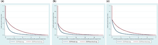
(a–c) Health payment budget share against cumulative percentage of Households Ranked by decreasing budget share in rural, urban and all areas of Bangladesh, year 2010.
Descriptive statistics shows that households with female and elderly head faced more CHE incidences at both 10 and 25% threshold levels. Further, household heads with higher educational levels had lower CHE incidences. While 14.7% households with 1–10 years of schooling faced CHE, only 9.9% households faced the same with 10+ years schooling at threshold level of 10%. The pattern remained same when CHE estimated at 25% threshold level. Presence of old-age people (65 years and above) in household increased the CHE incidence from 13.2 to 18.1%, while it increased from 13.6 to 14.4% in presence of children (under 15 years). Presence of reproductive age women in the households increased CHE incidence rate from 12.9 to 17.0% at 10% threshold level. Further, households with five members or more faced higher rate of CHE incidence than those households with one to two or three to four members. Similar patterns found when CHE incidence rates were estimated at 25% threshold level of non-food expenditure as well (Table 4).
Incidence of CHE by household characteristics, types of illness or symptoms and healthcare seeking behaviour
| Characteristics | Incidence of CHE | |
|---|---|---|
| 10% of total expenditure (95% Confidence Interval) | 25% of non-food expenditure (95% Confidence Interval) | |
| Gender of household head | ||
| Male | 13.8% (12.8%–14.8%) | 17.4% (16.3%–18.5%) |
| Female | 16.7% (14.6%–18.9%) | 18.9% (16.7%–21.2%) |
| Age of household head | ||
| Under 60 years | 13.8% (12.8%–14.9%) | 17.0% (16.0%–18.1%) |
| 60+ | 16.3% (14.3%–18.4%) | 20.8% (18.6%–23.1%) |
| Years of schooling of household head | ||
| 0 year | 14.6% (13.3%–15.9%) | 19.9% (18.5%–21.4%) |
| 1–10 year | 14.7% (13.5%–16.1%) | 16.3% (15.0%–17.6%) |
| 10+ | 9.9% (7.8%–12.4%) | 9.6% (7.6%–12.0%) |
| Household member’s characteristics | ||
| Presence of old age (65 years and above) | ||
| No | 13.2% (12.3%–14.3%) | 16.4% (15.4%–17.6%) |
| Yes | 18.1% (16.3%–20.1%) | 22.3% (20.3%–24.5%) |
| Presence of child (under 15 years) | ||
| No | 13.6% (12.1%–15.3%) | 16.0% (14.5%–17.8%) |
| Yes | 14.4% (13.3%–15.4%) | 18.0% (16.9%–19.2%) |
| Presence of reproductive age women | ||
| No | 12.9% (11.9%–13.9%) | 16.1% (15.0%–17.2%) |
| Yes | 17.0% (15.4%–18.8%) | 20.9% (19.1%–22.8%) |
| Household size | ||
| 1–2 persons | 14.5% (12.5%–16.8%) | 18.3% (16.0%–20.9%) |
| 3–4 persons | 13.1% (12.0%–14.3%) | 15.9% (14.7%–17.1%) |
| 5 persons or more | 15.2% (13.9%–16.6%) | 19.1% (17.7%–20.6%) |
Table 5 shows the results from multivariate analysis for predicting the effect of demographic and socioeconomic characteristics on CHE. It was observed in model 1 (CHE with threshold level at 10% health expenditure of total consumption expenditure) that the likelihood of CHE was higher among the households with female, lower number of schooling years of household heads and presence of reproductive age women. Urban households and those in richest socioeconomic quintile had significantly lower rate of CHE.
Determinants of CHE in Bangladesh
| Variables | Description | Model 1 | Model 2 |
|---|---|---|---|
| (Dependent = 10% of total expenditure) | (Dependent = 25% of non-food expenditure) | ||
| OR (95% confidence interval) | OR (95% confidence interval) | ||
| Gender of household head | Female (Ref = Male) | 1.216* (1.046,1.414) | 1.057 (0.914,1.222) |
| Age of household head | 60 + (Ref = Under 60 years) | 0.941 (0.794,1.114) | 0.973 (0.830,1.141) |
| Years of schooling of household head | 1–10 year (Ref = 0 year) | 1.171** (1.044,1.313) | 1.013 (0.910,1.128) |
| 10 + (Ref = 0 year) | 0.915 (0.731,1.145) | 0.756* (0.600,0.951) | |
| Household with old age member (65 years and above) | Old age (Ref = household without old age member) | 1.242** (1.056,1.461) | 1.268** (1.088,1.479) |
| Household with child member (under 15 years) | Child (Ref = Household without child member) | 1.114(0.950,1.307) | 1.260** (1.080,1.471) |
| Household with reproductive age women (15–49 years) | Reproductive age women (Ref = Household without reproductive age women member) | 1.261**(1.098,1.449) | 1.287***(1.129,1.467) |
| Household size | 3–4 persons (Ref = 1–2 persons) | 0.877 (0.712,1.081) | 0.871 (0.714,1.063) |
| 5 persons or more (Ref = 1–2 persons) | 1.031 (0.822,1.293) | 1.048 (0.844,1.300) | |
| Area | Urban (Ref = Rural) | 0.705*** (0.618,0.804) | 0.725*** (0.640,0.822) |
| SES quintile | 2nd (Ref = Poorest) | 0.973 (0.832,1.136) | 0.789*** (0.689,0.905) |
| 3rd (Ref = Poorest) | 0.942 (0.802,1.106) | 0.678*** (0.587,0.783) | |
| 4th (Ref = Poorest) | 0.961 (0.809,1.142) | 0.581*** (0.494,0.682) | |
| Richest (Ref = Poorest) | 0.775* (0.627,0.958) | 0.389*** (0.316,0.478) | |
| Constant | 0.130***(0.0980,0.174) | 0.247*** (0.188,0.324) | |
| N | 12,219 | 12,219 | |
| Log likelihood | −4972.1 | −5466.9 | |
| LR Chi2 (14) | 151.1 | 394.6 | |
| Prob > Chi2 | 0.000 | 0.000 |
***, ** and * denote the significance levels at 0.1%, 1%, 5% and respectively.
Estimation model 2 (CHE with threshold level at 25% health expenditure of total NFE) in Table 5 suggested that higher number of schooling years of household heads and higher socioeconomic status reduced CHE significantly. On the contrary, presence of elderly members (65 and above) and children (under 15 years) and female members at reproductive age (15–49 years) resulted in higher CHE rate.
Impact of poverty
A graphical presentation of impact of OOP payments on poverty is presented in Figure 2. Households were ranked from poorest to richest along using total consumption expenditure in the y-axis. Poverty-line was used for capturing the impact.
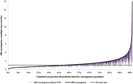
Poverty impact on Pen’s Parade non-health per capita expenditure using national poverty line.
We observed that a number of individuals, which were above the poverty-line, fall later below after subtracting the OOP payments from their total household consumption expenditure. Most such falls occurred in marginal populations, i.e. those who were just above the poverty-line.
The change in poverty headcount due to OOP expenditure is presented in Table 6. The poverty headcount was 37.8% considering total household consumption expenditure with gross OOP spending. It increased to 41.3% when total expenditure was calculated without OOP payments.
Measures of poverty based on consumption gross and net spending on health care
| Head count with gross OOP payments | Head count without OOP payments | Difference | ||
|---|---|---|---|---|
| Absolute | Relative | |||
| Poverty headcount | 37.8% | 41.3% | 3.5% | 9.1% |
| Standard error | 0.008 | 0.008 | 0.002 | |
| Poverty gap | 819.4 | 922.5 | 103.1 | 12.6% |
| Standard error | 21.5 | 22.6 | 4.2 | |
| Normalized poverty gap | 10.9% | 12.3% | 1.4% | 12.6% |
| Standard error | 0.003 | 0.003 | 0.001 | |
This 3.5% increase in the poverty headcount corresponds to 5.1 million individuals. The normalized poverty gap indicated the average amount by which the resources fall short of the poverty line as a percentage of that line. The normalized poverty gap increased from 10.9 to 12.3% if OOP payments were deducted from total expenditure.
Discussion and conclusions
This study observed that CHE had been incurred by 14.2% of households nationally, but it was more concentrated in rural (16.3%) than urban (8.6%) populations and also more concentrated in households with lower socioeconomic status. It was further found that several demographic and socioeconomic characteristics contributed to CHE. It was further found that 3.5% of total population fell into poverty annually due to OOP spending for healthcare, which corresponds to economic impoverishment of 5 million people in Bangladesh.
Findings from this study were in the same line as some previous studies in Bangladesh (van Doorslaer et al. 2007; Rahman et al. 2013; Hamid et al. 2014). Rahman et al. (2013) found by analysing urban people from a metropolitan city of Bangladesh that 9% of households face financial catastrophe due to health spending and such catastrophe is four times higher in poorest households than the richest ones. Our findings in this regard are similar, implying that 8.6% of urban population face financial catastrophe and it is 1.2 times higher among poorest households than the richest ones at the national level. Hamid et al. (2014), using data from rural people of low income group found that 3.4% people get into poverty due to OOP spending for healthcare. This study also suggested the similar findings while investigating poverty at the national level. Hamid et al. (2014) and Rahman et al. (2013) used data from year 2009 and 2011, respectively, which is almost the same period, i.e. 2010 of the data used by this study.
Van Doorslaer et al. (2007), using data from 2000, found that 15.6 and 7.1% of households in Bangladesh faced CHE considering 10% of THCE and 40% of NFE, respectively, as thresholds (Van Doorslaer et al. 2007). The authors observed that richer households experienced CHE more often. However, this study using data from 2010 found that poor households experienced more CHE. Some other countries, for instance, China, Nepal, Vietnam, Kenya, Georgia with negative or ∼0 value of concentration index showed the results in the same line as this study (Van Doorslaer et al. 2007).
It should also be noted that estimation techniques of measurements are different in different studies. For instance, households were placed into socioeconomics classes using alternative measurements, like, household consumption expenditure or asset index. Choosing asset quintiles for classifying households into socioeconomic groups in this study could be supported by arguments from O’Donnell et al. (2005), who pointed out in estimating CHE that using consumption expenditure as one of the explanatory variables in an economic model can lead to endogeneity problems (O’Donnell et al. 2005). The usage of asset quintiles for socioeconomic classification, as was done in this study, could avoid such a problem (Joglekar 2008). In an earlier study, poverty was measured using US$1.08 as a threshold (van Doorslaer et al. 2006), and CBN in our study. The CBN method, which was used in Bangladesh for estimating the poverty line, was more appropriate since the local price level of household consumptions are considered (BBS 2011).
Unlike previous studies in Bangladesh, we analysed the data at national level and also for urban and rural areas separately. In addition to the studies of Hamid et al. (2014), Rahman et al. (2013) and van Doorslaer et al. (2007), this study provided a more complete understanding of the impact of OOP for healthcare on CHE and poverty by disaggregating the analyses into urban and rural areas. The major limitation of this study is that it is based on cross-sectional data. Ideally, longitudinal data would be used to estimate the causal effect of impoverishment resulting from OOP for healthcare. This would allow one to identify how spending on non-medical goods and services changes following a health shock (Sauerborn et al. 1996).
We found sociodemographic and economic gradients in CHE rates though it varied to some extent when we applied two different definitions (10% health expenditure of total household consumption expenditure and 25% health expenditure of total NFE as CHE thresholds). The effects of demographic and socioeconomic variables that were found in the analyses were mostly expected.
Bangladesh has made significant progress between 2005 and 2010 by reducing the poverty rate from 40.0 to 31.5% (BBS 2007, 2011). The study of van Doorslaer et al. (2006) found that OOP contributed to poverty by 3.8% in 2000, and this study observed a corresponding rate of 3.5% in 2010 (van Doorslaer et al. 2006). This implies that while poverty in general reduced by a higher rate (from 40.0 to 31.5%), we observed just a slight reduction in poverty attributed to OOP for healthcare. Healthcare financing methods of Bangladesh should concentrate on finding alternative financing methods than OOP for reducing the probability of CHE and consequently poverty. Pre-payment mechanisms, like social health insurance, which are often recommended by international organizations, e.g. the WHO and the World Bank, should be applied in Bangladesh as a remedy for reducing financial risk and poverty attributed to OOP healthcare spending (WHO 2010). The Government of Bangladesh developed the healthcare financing strategy for addressing social protection in order to achieve universal health coverage (MoHFW 2012). The strategy recognized the impact of OOP healthcare financing mechanism on financial risk and poverty and consequently recommended reduction of OOP as a share of total health expenditure from 64 to 32% in 20-year period (2012–2032) and applying prepayment mechanisms, like social health insurance, tax funding, community-based health insurance, more. Findings from this study would be supportive to the healthcare financing strategy of the Government for monitoring the progression towards universal health coverage in Bangladesh.
Acknowledgements
The authors like to thank Andrew Mirelman and participants of “Measuring UHC meeting” for their valuable comments on the manuscript and presentation of study results. Gratitude goes also to Dr. Abbas Bhuiya, Dr. Sadia Chowdhury, Dr. Syed Masud Ahmed and Dr. Nurullah Awal for their cordial cooperation for conducting the study. Thanks also go to Andrew Mirelman also for language editing. International Centre for Diarrhoeal Disease Research, Bangladesh (icddr,b) gratefully acknowledges the following donors who provided unrestricted support: the Government of the People's Republic of Bangladesh; Global Affairs Canada (GAC); the Swedish International Development Cooperation Agency (Sida), and the Department for International Development (UK Aid).
Funding
This project has been funded in whole from Rockefeller Foundation. The Centre of Excellence for Universal Health Coverage of icddr,b and James P Grant School of Public Health acknowledge with gratitude the commitment of the funder to its research efforts.
Conflict of interest statement. None declared.
Ethical approval
This article has been prepared using secondary data (Household Income and Expenditure Survey of Bangladesh) from Bangladesh Bureau of Statistics. Thus, no ethical approval is required separately for this study.
