


Abstract
Aging is a complex phenomenon, with numerous simultaneous processes that interact with each other on a moment-to-moment basis. One way to quantify the interactions of these processes is by measuring how much a process is similar to its own past states or the past states of another system through the analysis of recurrence. This paper presents an introduction to recurrence quantification analysis (RQA) and cross-recurrence quantification analysis (CRQA), two dynamical systems analysis techniques that provide ways to characterize the self-similar nature of each process and the properties of their mutual temporal co-occurrence.
We present RQA and CRQA and demonstrate their effectiveness with an example of conversational movements across age groups.
RQA and CRQA provide methods of analyzing the repetitive processes that occur in day-to-day life, describing how different processes co-occur, synchronize, or predict each other and comparing the characteristics of those processes between groups.
With intensive longitudinal data becoming increasingly available, it is possible to examine how the processes of aging unfold. RQA and CRQA provide information about how one process may show patterns of internal repetition or echo the patterning of another process and how those characteristics may change across the process of aging.
Recurrence Quantification for the Analysis of Coupled Processes in Aging
Life-span developmental theory highlights the dynamic nature of aging, with reciprocal influences among processes manifesting at both different levels of analysis and different time scales (e.g., Baltes, Lindenberger, & Staudinger, 2007; Gottlieb, 2007). These processes may show combinations of repeated, habitual patterns, novel responses to external inputs, and both sudden and gradual changes in their dynamics. That is, changes in my mood this week may mirror the pattern of changes observed next week but may be totally different from the patterns that appear 2 weeks from now. Similarly, interactions with others may show give-and-take patterns of mirroring, where one spouse’s mood or one conversant’s movement echoes the other’s. Further, these cycles may show nonstationarity, where the pattern of self-similarity changes, for example, with habit or across the process of aging.
Modern data collection tools such as daily diary studies, computer-vision techniques, and social media monitoring make it possible to collect intensive longitudinal data that can show highly nonlinear dynamics, sudden shifts in regime, and different patterns of self-similarity. As these data become increasingly available, we must turn to more dynamical techniques to understand the processes at work and how they evolve and change across time and age. In this paper, we present one such dynamical technique—recurrence quantification analysis (RQA) and cross-recurrence quantification analysis (CRQA)—as an approach to model dynamic patterns in behavioral science data.
RQA (Eckmann, Kamphorst, & Ruelle, 1987) and CRQA (Zbilut, Guiliani, & Webber, 1998) permit researchers to answer questions about the repeating patterns that people follow, and the way that those patterns change across time. For example, as people age, do the patterns of stressors they encounter become more consistent? Does caregivers’ affect mirror the patterns of affect in those they care for? Or, foreshadowing the example in this paper, are older adults more predictable in the way that they respond to each other’s movements in conversation? Do those differences in patterning hold when talking to younger adults? We expect that these techniques will be of specific benefit to research about aging because they allow researchers to examine the patterns of everyday life and the way that those patterns change across the life span without the need for specific strong hypotheses or mathematical models about the specific nature of those patterns.
The broad applicability of these methods to almost any type of time series data make them suitable for cases, such as ordinal data, where other time series models of dynamics may be biased (e.g., Hu & Boker, 2016). Tools like these are especially useful with the emergence of dense data collection because they create opportunities for both mathematical confirmation of theory driven hypotheses about patterns of change over time and for theory-free visual exploration of data to assist in the generation of new hypotheses and new theories based on existing data sets.
We first introduce the Theoretical Background necessary to understand recurrence relationships and then introduce The Present Study. In Methods, we present the primary idea of recurrence and the recurrence plot. We specifically focus on the way that recurrence, determinism, and changes in dynamical regimes can be seen on a recurrence and cross-recurrence plot, and on the characteristic measures reported by RQA and CRQA analyses. In Data Analysis, we describe the process of applying RQA and CRQA to example data, briefly reporting the qualitative Results revealed and indicating the statistical methods appropriate to their use in hypothesis testing. In the Discussion, we interpret the findings from our analyses and the Future Work in the application of these methods.
Theoretical Background
Dynamic Patterns in Behavioral Science Data: Self-Similarity and Symmetry
In the study of aging, we frequently use linear or piecewise linear models to approximate change over a long period of time, averaging over or ignoring variability at shorter time scales. Yet in practice, the process of aging is nonlinear, moving in cycles and bursts. For example, a participant’s motivation may similarly oscillate, showing a pattern where high-stress weeks results in burnout and a cycle of low motivation followed by a recovery period. The participant’s behavior at a given time point most likely resembles a pattern of behavior they have previously exhibited. Their behavior shows recurrence of past patterns, a type of self-similarity.
These types of repetition can also be influenced by outside factors or can show temporal symmetry with other processes, that is, they may show behavior that is similar to the other process but which either leads or follows it (Brick & Boker, 2011). For example, depression and rates of suicide may be related to cycles of weather (Partonen et al., 2004; Boker, Leibenluft, Deboeck, Virk, & Postolache, 2008). In conversation, patterns of mirroring in posture and head movement are associated with traits and outcomes including perceived participant gender (Boker et al., 2011; Theobald et al., 2009), empathy and rapport (e.g., Duffy & Chartrand, 2015), and clinical outcomes (Ramseyer, 2014; Ramseyer & Tschacher, 2011).
RQA and CRQA provide methods to unpack otherwise inaccessible dynamic characteristics of the system, providing a means of measuring self-similarity and between-construct or between-person symmetry across time. RQA and CRQA allow us to model traits such as the determinism of a system, the dimensionality or complexity of its dynamics, and the amount of repetition and patterning it holds. They also provide tools to assess repeated patterns, sequences, and regime shifts both quantitatively and qualitatively. Notably, RQA and CRQA are robust to nonlinearity and some forms of nonstationarity within the system (e.g., within an individual or a dyad across time). These methods also produce readily interpretable visualizations that provide insight into the characteristics of changing systems. To demonstrate the applicability of RQA and CRQA to behavioral science data, we present an example of age-related differences in head-movement patterns during conversation.
The Present Study
In our applied example looking at head movements in conversational interaction across age groups, we examine both individual RQA plots and dyadic CRQA plots for several example conversations and we highlight the statistical tests that can be used to test hypotheses related to the RQA and CRQA metrics.
In our example data, we hypothesize that in conversation, older adults may be less able to promptly and directly replicate the movements of their coconversants. As a result, we hypothesize less predictability and less repetition in conversations among older adults. Second, we hypothesize that there will be higher levels of synchrony in conversations where conversation partners belong to the same age group due to differences in behavioral style and movement speed. We use the metrics from RQA and CRQA to examine a subset of conversations and to quantify the differences between younger and older adults in this small sample. We provide both qualitative indicators and quantitative measurements of our outcome measures and we indicate the statistical methods appropriate to test our hypotheses.
Methods
We first describe the RQA and CRQA methods and then present our example study.
Recurrence and Recurrence Plots
The methods introduced in this paper rely first and foremost on the concept of recurrence. Recurrence is easiest to think about in a categorical context. Assume we have coded a video of a participant’s facial expression. At each time point in the video, we have indicated whether the participant shows a smile (S), a frown (F), open mouth (O), or one of five specific speech movements (A, B, C, D, and E). In this simple space, we can define the recurrence between two time points as an equality relationship: If and only if the person’s expression at both time points is the same type of expression, then we consider the two points recurrent.
RQA both operates by computing the recurrence of each time point or short sequence in the time series with every other point or series in the same series. We can visualize these recurrence relationships by laying out a grid with time in the sequence moving forward along both the X and Y axes. In this simplified case, we shade those (x,y) coordinates where time point x is recurrent with time point y, as shown in Figure 1. This is a simple form of recurrence plot.
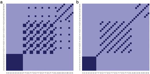
Recurrence plots of a categorical time series. (a) The recurrence plot of a categorical time series. A dark point at (x,y) indicates that time point x and time point y show the same expression. (b) The same plot with an embedding dimension of 3 and a delay of 1.
In Figure 1, time can be considered to progress from the bottom left corner, flowing both upwards and to the right simultaneously, with the solid diagonal line in the center indicating synchrony. Immediately obvious is the block-like structure of the plot. The dark block in the lower left is an area of minimal movement in which the participant smiles without change—it is dark because each second is the same as (and therefore recurrent with) every other. Around 20 s into the conversation, the participant’s mood changes suddenly. The large empty area on the lower and left side of this segment indicates that this next block is not at all recurrent with the first 20 s but the checkerboard pattern in the center of the plot between 20 and 40 s on both axes is typical of a regular pattern of short oscillations among states; here, we see the sequence FFOC, repeated several times. The last 20 s of both axes shows a different repeating pattern: ABCDE. The longer, sparser diagonals in this section indicate the repetition of this longer, less repetitive sequence. The sparse dotted pattern in the off-diagonal elements shows that there is some commonality (Cs) between the FFOC and ABCDE patterns.
In a dyadic or multivariate context, the concept of cross-recurrence is similar. Instead of asking whether we have seen a given pattern or location at a different point in time in the same sequence, we now ask when and whether this pattern appears in the other sequence. For example, a participant in a daily diary study might report several days of rising anxiety overlapping with several days of rising stress. This lead-follow relationship, where one time series (e.g., stress) follows the pattern of another (e.g., anxiety), is an example cross-recurrence.
This article introduces RQA and its dyadic form, CRQA for the study of aging by approaching it from the perspective of a user—a scientist wishing to use RQA and CRQA recurrence plots to understand their data. In this context, we propose two of the following primary ways to apply RQA/CRQA:
Qualitative examination of recurrence plots. Recurrence plots visualize the recurrence relationships within a data stream. Direct examination of these plots provides a quick, qualitative view of where self-similar relationships appear, can show evidence of more or less predictable behavior and indicate areas where potential regime changes occur. All the information needed to reconstruct the data is displayed in the recurrence plot (Tanio, Hirata, & Suzuki, 2009).
Statistical modeling of hyperparameters and characteristics of the recurrence plot. The recurrence plot carries information about the amount of recurrence, the proportion of deterministic behavior, and the longest recurrent sequences in the data set. These can be modeled through traditional analysis tools to find group differences or relationships. Provided their assumptions are met, standard techniques like or analysis of variance (e.g., Tolston, Ariyabuddhiphongs, Riley, & Shockley, 2014) can be used; if assumptions are not met, comparisons can still be made with nonparametric approaches, or using bootstrap- or surrogate-data-based methods to approximate confidence bounds (e.g., Schinkel, Marwan, Dimigen, & Kurths, 2009).
Before embracing the method of RQA and CRQA, we first discuss its history, its requirements, and the underlying mathematics.
History of RQA and CRQA
RQA and CRQA are methods developed to measure and visualize patterns in time series data. RQA was first presented by Eckmann et al., 1987 in the dynamical systems and physics literature, where it has remained popular due to its ability to handle complicated nonlinear dynamical systems showing chaotic, fractal, and multifractal structure. While the concepts of fractal and multifractal structure are beyond the scope of this tutorial, there is some evidence that many human systems show evidence of multifractal structure (e.g., Shimizu, Barth, Windischberger, Moser, & Thurner, 2004) and that the breakdown of such structure is an important indicator of a failure of the system (Ivanov et al., 1999). We hope that RQA will provide one additional avenue toward more complicated multifractal models of behavior. CRQA was developed 11 years later by Zbilut et al., 1998 and has been praised for its ability to detect small signals, even in systems with large amounts of noise.
RQA and CRQA have been used extensively in other fields to monitor nonstationary systems for purposes like detecting epilepsy (Thomasson, Hoeppner, Webber, & Zbilut, 2001), locating homologous proteins (Yang, Tantoso, & Li, 2008), exploring the relationship between El Nino and rainfall (e.g., Marwan & Kurths, 2002) and identifying regime changes in environmental data across time (e.g., Zaldívar, Strozzi, Dueri, Marinov, & Zbilut, 2008; Facchini, Mocenni, Marwan, Vicino, & Tiezzi, 2007). Within the behavioral sciences, RQA and CRQA have been used on data ranging from eye-tracking of individuals and dyads (Anderson, Bischof, Laidlaw, Risko, & Kingstone, 2013; Dale, Kirkham, & Richardson, 2011; Richardson, Marsh, & Schmidt, 2005), heart rate (Konvalinka, Xygalatas, & Bulbulia, 2011) and heart rate variability (dos Santos, Barroso, de Godoy, Macau, & Freitas, 2014), to EEG (Ouyang, Li, Dang, & Richards, 2008), to body movement (Tolston et al., 2014), to linguistic data (Dale & Spivey, 2006), although great potential exists for applications in other areas, especially for interaction (Fusaroli, Konvalinka, & Wallot, 2014; Shockley & Riley, 2015).
Data Requirements
RQA and CRQA make very few assumptions about the data. These analyses do not require any specific knowledge or assumptions about the underlying model (Zbilut et al., 1998). Notably, they do not assume either linearity or strict stationarity and so function on systems whose dynamic and static characteristics change drastically throughout the measurement interval. Specifically, RQA and CRQA require that the definition of “similarity” in time points and time series, hold throughout the entire sequence. For a categorical variable, this simply requires that the meaning of the categories holds constant across groups. For a continuous-valued time series, this means that a distance between any two values keeps its meaning regardless of the location or time. Notably, almost any repeated pattern of behavior may be found by RQA, regardless of the time span between them. However, if two sequences show similar patterns of change but differ in mean (e.g., sequences 1234 and 6789), their similarity may not be noticed by standard RQA, although extensions through normalization and windowing may address this concern.
Mathematically, RQA and CRQA can be computed for sequences of any length. To provide interpretable results, however, it is helpful to have data that meet some minimum requirements. For example, to capture the recurrent nature of a pattern, the time series must be long enough that the pattern occurs at least twice. Similarly, the data must be sufficiently dense (i.e., recorded with a small enough time between measurements) that the pattern can be distinguished from noise.
To illustrate the concept of sufficient density, consider the following examples. Drug use might be rated using a daily Likert-like measure asking about drinking behavior each day over the course of a month. At this rate of measurement, it would be possible to see weekly repeating patterns (e.g., higher use on weekends followed by lower use on Monday and Tuesday). It would be more difficult, however, to see biweekly paycheck-based patterns and impossible to spot within-day patterns. By contrast, the repetitive motion involved in a head-shake would not be visible at all if head location was recorded on even a minute-to-minute basis; measurements separated in tenths or hundredths of a second would be required. To measure seasonal variability in affective state, once-monthly assessments might be required over several years before the pattern was evident. In each case, it is important to match the timescale of measurement to the timescale of the process (see Gerstorf, Hoppmann, & Ram, 2014 and Hollenstein, Lichtwarck-Aschoff, & Potworowski, 2013 for examples of timescale-aware measurement).
In practice, a repeating pattern can be detected by RQA and CRQA and distinguished reliably from noise if the time series is measured rapidly enough that three or four measurement occasions fall within each repetition of the pattern and shows two repetitions of the whole pattern. Note that these represent minimal requirements; more repetitions of the pattern or more measurements per repetition permit more robust and precise estimation. In general, more noise in the data will reduce the ability to detect patterns; more data may be required for noisier data.
The most common problem with time series data is missingness, which can be handled by many but not all RQA/CRQA software packages. In cases where missingness cannot be handled automatically, linear or spline interpolation, a locally weighted regression smoother (loess; Cleveland & Devlin, 1988) or other standard time series imputation tool may be appropriate (see e.g., Steffen, Sarda, Artz-Beielstein, Zaefferer, & Strok, 2015).
RQA and CRQA work best when a given difference carries the same meaning consistently. That is, the visualization may be somewhat skewed in the presence of, for example, soft ceiling effects or logarithmic scales, where the importance of a unit change may be less impactful in some areas. As a result, it may be helpful to apply transformations, such as normalization or log-transformations to the data before applying RQA and CRQA. For models such as EEG where scale is unknown or may change over the sequence, other transformations such as permutation orderings (e.g., Schinkel, Marwan, & Kurths, 2007) may be better.
Mathematics of RQA and CRQA
Mathematically, recurrence can be thought of as a measure of similarity between the elements of two potentially multivariate time series. In the case of categorical data, the similarity relationship is simple: items are either equivalent or they are not. For continuous data, RQA treats each time point in a sequence as a point on a number line. Points are recurrent if they are within some predefined distance or boundary, called the cutoff radius (r). If the data are multivariate, they are treated as points on a plane or in a higher dimensional space. In each case, if the Euclidean distance between the points is smaller than the cutoff radius, the two time points are said to be recurrent. If the distance is larger, then they are not recurrent. The formal definition for the recurrence value of two potentially multivariate time points x and y given a cutoff radius r is:
It is also possible to use color or shading to draw the distance between points directly on the plot itself. Figure 2a and b shows the same RQA plot. The thresholded binary recurrence plot in Figure 2a provides a simplified picture and shows the results of recurrence analysis. The contour plot in Figure 2b provides a more nuanced view of the relationship, which can be useful for qualitative interpretation.
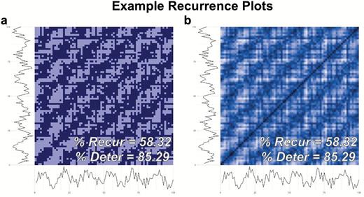
Recurrence plots of a noisy sine wave. (a) A binary recurrence plot. A dark point at (x,y) indicates recurrence between time point x and time point y. (b) A contour plot of the recurrence relationship. Lighter colors indicate that a larger cutoff radius is required before the point is considered recurrent.
CRQA is the same as RQA, but compares each time point of one time series with every time point of another. The plots created from this are called cross-recurrence plots. Figure 3 shows examples of both recurrence plots and cross-recurrence plots.
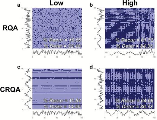
Top: Two recurrence plots. (a) Low recurrence and low determinism. (b) Higher recurrence, higher determinism, and evidence of regime change. Bottom: Two cross-recurrence plots. (c) Low cross-recurrence. (d) High cross-recurrence. CRQA = cross-recurrence quantification analysis; RQA = recurrence quantification analysis.
Hyperparameters of RQA/CRQA
Differences in the ways that behavioral systems function can lead to differences in the way that recurrence is computed and understood. Differences in the amount of measurement noise and differences in the complexity of the system being modeled can lead to differences in what points are close enough to be considered “recurrent”. These differences between systems can be addressed by manipulating the hyperparameters of RQA and CRQA. The first hyperparameter, radius, represents the cutoff distance for recurrence, as explained earlier. Two others, embedding dimension and delay, allow a more direct analysis of sequences of recurrent behavior. The choice of hyperparameters can have an important effect on the understanding of a recurrence plot.
Frequently in the determination of repeated behavior, we are interested in finding out not only when behavior at a given time point is similar but also when the path to reach those points is similar. We may therefore consider two time points to be recurrent only if they both have similar values and took similar paths to get to that point. To do this using RQA and CRQA, we use a process called time delay embedding (see, e.g., von Oertzen & Boker, 2009 for a more complete discussion). Time delay embedding simply adds history to each row, so that instead of a row holding only the current value Xt, it holds a vector of m past time points, spaced out at some delay d [Xt, Xt–d, Xt–2*d, ..., Xt–(m−1)*d]. All these elements are then compared as though the sequence were multivariate when recurrence is determined. With a three-dimensional embedding and a delay of 1, two points would be considered recurrent if the sequences looked similar over a window of three consecutive measurements; with a two-dimensional embedding and a delay of five, time point 10 would be recurrent with time point 20 only if the vector (X10, X5) matched (X20, X15). Note that this embedding process requires a window of data elements for each row. It therefore reduces the number of available rows by (m-1)*d, although in most practical cases this reduction is small compared with the number of total rows. Note that using an embedding dimension greater than 1 adds an additional assumption that the embedding dimension is stationary, such that the value chosen is appropriate across the entire span of the data. Windowed (C)RQA may be more appropriate in cases when this assumption does not hold (Coco & Dale, 2014).
The application of time delay embedding changes the interpretation of the recurrence plot in important ways. Instead of simply indicating that two time points resemble each other, recurrence of a time delay embedded time series indicates that the sequence has followed a similar pattern of change to arrive at the same point, that is, they have arrived at the same point in the same way. Embedding can be helpful in understanding the differences between cyclical behaviors, chance outliers, and other phenomena. For example, consider Figure 1b, which shows the same pattern as Figure 1a but with an embedding dimension of 10 and delay of 1. Notice in particular that only the main diagonal is recurrent at the areas of change between regimes, such as near second 20, that the block-and-diagonal structure of the center block has become a clean diagonal structure, and that the sparse points in the off diagonal have disappeared. Points at each of those locations are identical but the C in ABCDE did not follow the same path as the C in FFOC and is therefore no longer considered recurrent. This type of embedding is especially helpful in finding sequential patterns or dynamics in the data.
When comparing across individuals, the choice of embedding dimension, delay, and cutoff radius can either be chosen to be unique for each individual or dyad (similar to a random-effects approach) or fixed across all (a fixed-effects approach; see also Zbilut & Webber, 1992). We recommend maintaining a low-dimensional embedding, as these have been shown to capture all the information required to model many dynamical systems (e.g., Iwanski & Bradley, 1998; March, Chapman, & Dendy, 2005). Noisier systems are more likely to show spurious recurrence at high embedding dimension; so, dimensionality below 10 is recommended for behavioral data, whereas for biological data with relatively less noise, dimensions up to 20 may be viable (Webber, Marwan, Facchini, & Giuliani, 2009).
The delay parameter determines the timescale over which the embedding operates. If a specific periodic pattern is of interest, the delay can be chosen based on the state space of the expected pattern (usually one fourth of the duration of the pattern). However, Webber & Zbilut (2005) recommend setting delay to 1 if interested in finding sequential patterns (where one movement immediately follows another).
In cases where there is little background theory, these hyperparameters can be optimized using data-driven approaches that maximize important quantities. Radius, for example, is often chosen to minimize the fragmentation and thickness of diagonal lines in the RQA plot (e.g., Matassini, Kantz, Holyst, & Hegger, 2002), which balances the ability to find recurrent sequences with the ability to distinguish them from the surrounding details. Other approaches select a radius to target a specific range of Recurrence Rates (Webber & Zbilut, 2005) or as a fraction (often 10%–30%) of the maximum distance between points. Similarly, embedding dimension may be approximated based on the dimensionality of the underlying dynamical system using approaches such as false nearest neighbors, although other methods exist (Yonemoto & Yanagawa, 2001). Briefly, false nearest neighbors increase the embedding until increasing it ceases to make large differences in which points are near each other (see Kennel, Brown, & Abarbanel, 1992 for more). Delay is often selected to maximize mutual information between the two time series in the plot (Webber & Zbilut, 2005). Finally, graphical methods can be used to examine sensitivity to these hyperparameters, and parameters can be selected on those grounds (Marwan & Webber, 2015).
Application 1: Qualitative interpretation of recurrence plots
Although we cover only a few general concepts here, a wide array of features can be gleaned by examination visual of the recurrence and cross-recurrence plots (see Marwan & Webber, 2015 and Marwan & Kurths, 2005 for more complete coverage). The plots in Figure 2 visualize the recurrence relationships within a single simulated time series drawn along each axis. Our example here is simulated from a linear oscillator and so shows cycles of highs and lows in regular intervals, similar to a swinging pendulum.
One obvious feature of the recurrence plot in Figure 2a (also visible in the contour plot in Figure 2b) is the diagonal line stretching from the lower left corner of the plot to the top right corner. This central main diagonal represents synchrony, where each point in the time series is compared precisely to itself (and, of course, is equal). Diagonal segments parallel to the primary diagonal each represent a recurrent sequence, where the same pattern is followed. For example, the long band in Figure 2 sitting approximately 20 time points above the main diagonal indicates that the sequence shows self-similarity at a period of about 20 s. Diagonal segments perpendicular to the main diagonal indicate that the sequence shows the opposite of previous behavior, like a pendulum swinging back the way it came, whereas diagonal segments with other slopes may be indicative of similar sequences occurring at slightly different speeds.
Because the time series (in this case, a simulated regular oscillator with noise) consists of a single repeating pattern, bands of dark recurrent points are visible parallel to the diagonal that span the entire figure. Therefore, at every time point, a similar value will be found roughly twenty seconds later. The consistent periodicity of these plots means that the pattern of dynamics is repeated regularly. Slow or sudden disruption of the periodicity of this pattern indicates slow or sudden changes in the dynamics of the system.
Figure 3 shows four recurrence plots that illustrate how RQA and CRQA can answer questions about pattern recurrence and determinism. The top row of Figure 3 (Figure 3a and b) contains RQA plots that each show the recurrence pattern of one sequence of behavior, whereas the bottom row (Figure 3c and d) contains CRQA plots that each show the recurrence relationship between a pair of sequences. Plots in the left-hand column (Figure 3a and c) show systems with low recurrence and low determinism (predictability), as evidenced by the relative rarity of dark patches and the relatively sparse horizontal, vertical, and diagonal line structures. By contrast, the right hand column (Figure 3b and d) shows systems with high determinism and high cross-recurrence. The long, clear diagonal structures in Figure 3b (top right) indicate determinism in the form of long repeated patterns of behavior. By contrast, the long vertical and horizontal structures on the lower left and lower right plots (Figure 3c and d) indicate areas that are more deterministic because they exhibit minimal or slow change, where a large number of measurements fall close to each other.
One particular feature of note in Figure 3b (upper-right) is the sudden change in pattern in the upper right corner of structure of the plot, as opposed to the relatively consistent pattern in Figure 3d. This qualitative shift is indicative of a regime shift—a major change in the way that a process functions. Like in Figure 1a, which features three distinct dynamic regimes, this blockwise structure may also be visible through large white blocks, indicating a lack of recurrence between sections. These blocks show evidence that the pattern of recurrence has changed in a qualitatively noteworthy way. Long blank lines may also highlight rare events or rare sequences.
The same characteristic structures appear in the CRQA plots. Dark points indicating recurrence along the main diagonal are moments of synchrony, where both time series show similar behavior at the same time. Recurrent points above the diagonal indicate that the person or measure on the Y axis is repeating the movements of the person on the X axis some time later, whereas points below the diagonal indicate the opposite. This relationship of leads and lags can be collapsed into a diagonal recurrence profile (DRP), which is similar to an autoregression plot (see Main, Paxton, & Dale, 2016 or Dale, Warlaumont, & Richardson, 2011.
Application 2: Quantification of characteristics of the recurrence plot
RQA defines metrics characteristic to the recurrence plot (Webber et al., 2009), which provide quantitative measures of these same qualitative characteristics of recurrence and cross-recurrence plots. Although there are other measures that can be extracted from a recurrence plot, our discussion of RQA and CRQA focuses on three measures related to self-similarity and predictability: percent recurrence, percent determinism, and laminarity. These three measures capture a great deal of the information about the dynamics of change in the recurrent system. In fact, the measures obtained from RQA are sufficient to reconstruct the forces driving change in many dynamical systems (Tanio et al., 2009).
Percent recurrence is the ratio of recurrent points compared with the possible number of recurrent points. Higher proportions of recurrence mean that more values across time are similar to each other. In RQA, this represents a characterization of how much self-similarity appears in the data set and can be indicative of either common sequences or of a limited range of motion. In CRQA, the percentage of recurrence represents the proportion of each time series that is seen at some point in the other time series and provides a measure of temporal symmetry (Brick & Boker, 2011). Recurrence may occur either because a pattern of change is repeated, or because one or both time series show very little change across a span of time. Examination of the plot can help distinguish these qualitatively but other measures are needed to distinguish them quantitatively.
Percent determinism and laminarity distinguish these by computing the proportion of recurrent points falling specifically on upward diagonal line segments or vertical and horizontal line segments (Riley, Balasubramaniam, & Turvey, 1999). These can be quantified as
where rij is the recurrence at point (i,j), l is the length of a line, dmin is the minimum number of sequential points required to be considered a line (frequently 2) and H(l) is the number of diagonal (for determinism) or vertical/horizontal (for laminarity) lines of length exactly l on the plot (Sips, Witt, Rawald, & Marwan, 2016). High laminarity indicates areas of limited or smooth motion, high determinism is sensitive to any repeating or unmoving pattern.
A wide array of other characteristics can be derived from these plots, such as the entropy of line lengths, the trapping time (mean length of vertical/horizontal lines) of periods of minimal change, and many others (Fusaroli et al., 2014; Webber & Zbilut, 2005).
In CRQA, higher determinism indicates that one time series is more easily predicted by the past movements of the other time series. A more deterministic system shows more patterned behavior and is more predictable than a less deterministic one. Note that because RQA and CRQA are nonlinear methods, higher determinism does not mean a higher regression coefficient, nor even a higher autoregressive coefficient. In both RQA and CRQA, this determinism can have distinct theoretical implications. For example, we hypothesize here that older adults will be less able to integrate their own movements with those of their conversational partners. We expect older adults will mirror their conversational partners less often; therefore, they will show less recurrence and less determinism on a CRQA plot.
Data Source
To demonstrate RQA and CRQA in practice, we use a very minimal sample of four individuals and three conversations from a larger study on expressed emotions during conversations between unacquainted adults across the life span (in a paradigm similar to Boker, Staples, & Brick, under review).
Participants
Participants were four White men; two younger adults (aged 19, single, attending college) and two older adults (aged 69 and 72, married, and completed college). Younger adults received college course credit and older adults received $30 for their participation. Participants were fully informed of and consented to the audio and video recording prior to the study.
Procedure
Participants (four in each session) were randomly assigned to one of two adjacent rooms such that each room was assigned one younger and one older adult. Each participant took part three blocks, each with a unique social context (alone, younger partner, or older partner), presented in a randomized order. In each block, participants were asked to recount events from their life with a specific emotional context (angry, happy, or sad) for 2 min. Each individual therefore recounted a total of nine events, one for each emotion while alone, while talking via a videoconference link with a same-aged partner, and while talking via the same link with a differently aged partner. Participants were neither directed to nor cautioned against reminiscing about the same emotional event across social contexts. Participants in room one only conversed with the participants in room two (and vice versa) so that all recorded conversations were between unacquainted individuals. Participants completed questionnaires (e.g., demographics) when not conversing.
Participants were seated in a darkened room with their conversational partner appearing on a back projection screen directly in front of them. A small, unobtrusive video camera (Toshiba IK-HD1 720p 60HZ noninterlaced camera) hung from the ceiling at eye-height so that participants could engage in eye contact during the conversation. Audio was transmitted over headphones and recorded direct to disk by the V3HDs from two AKG overhead omnidirectional microphones, preamplified by a Yamaha 01V96 audio mixer.
A recorded audio prompt, transmitted via headphones, provided instructions about the emotional event to be discussed. Emotional context was counterbalanced across conversational dyads with a unique order for the conversations of an individual. After each conversation, participants completed a questionnaire about how they felt and how their partner felt (not presented in this study). Conversations selected randomly for this study were about past events during which the participants felt sad (both younger adults) or angry (younger and older adult and both older adults).
Analysis Procedure
In our substantive example, face location and facial expression points were first located on each frame of video data for the first minute of each conversation using a constrained local model (CLM) fitter from the CSIRO Face Modeling SDK (Saragih, Lucey, & Cohn, 2009) and a custom Face Modeling GUI (Brick, Braun, Harrill, & Yu, 2013). Local linear approximation (similar to Brick, Hunter, & Cohn, 2009; Rotondo & Boker, 2002) was applied to facial locations to extract an overall velocity of head movement at each time point. This transformation means that recurrence between movements requires only that the quantity of movement, not direction, be the same. As a result, one partner’s movement to the left will show recurrence with a corresponding movement to either the right or the left. Similarly, head-nodding will show recurrence with itself but also with any other repetitive movement of the same magnitude.
We applied RQA to the conversational head movements of each individual and CRQA to each dyadic conversation. Following the recommendations previously outlined, we use a delay of 1 and a data-driven optimized cutoff radius and embedding dimension for each plot. From each of these analyses, we created qualitative recurrence plots and computed laminarity, percent determinism, and percent recurrence.
We computed optimum hyperparameters and applied RQA and CRQA using the R statistical software package (R Core Team, 2016) crqa R package (Coco & Dale, 2014), and plotted using the R packages plyr (Wickham, 2011), dplyr (Wickham & Francois, 2015), and ggplot2 (Wickham, 2009). Data were rescaled and normalized during cross-recurrence computation to allow for differences in overall quantity of movement due to body size or age.
Results
Qualitative Exploration of Age Differences
Figure 4 shows the individual recurrence plots for each of the four participants. At a glance, it is clear that the younger participants showed denser areas of recurrence shown by the higher proportion of dark areas, more diagonal patterning, and longer diagonal lines, especially visible in comparing Figure 4a–c. Notice that while the overall structure is similar, the diagonal bursts in Figure 4a are shorter and less consistent than those in Figure 4c. The longer, darker areas especially notable in Figure 4d may indicate that younger adults may maintain a given position for longer. Older adults show shorter and more scattered line structures, indicating lower levels of recurrence and shorter repetitive sequences. This implies that the movements of younger adults showed more repetition, more stability and more consistent patterning. This might take the form of younger adults maintaining nodding behaviors for longer, or exhibiting long spans of immobility, which may be due to differences in a social characteristic like dominance, or a physical characteristic like muscle tone. By contrast, the movements of older adults were less repetitive and less predictable. Worthy of note is that all four plots show some larger blocks of sparser patterning, indicating regime changes in the data stream that may indicate changes in topic, or other large shifts in the structure of conversation, although this is much more pronounced in the younger adults, who show much less homogeneity in their RQA plots.
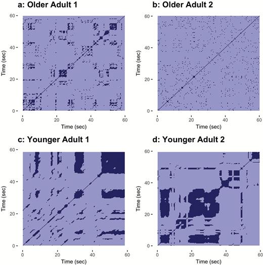
Example of recurrence plots of head movement from each of the four individuals in our pilot study. Older adults are shown in (a) and (b), younger in (c) and (d). Younger adults show higher recurrence in their movements.
Figure 5 shows the cross-recurrence plots for the first 2 min of the old-old (Figure 5a), old-young (Figure 5b), and young-young (Figure 5c) conversations. The old-old conversation (Figure 5a) shows a consistently sparse plot with limited diagonal structure and very few blocks of stability, implying less predictable and repetitive patterning in movements, which is reminiscent of white noise. The denser, darker blocks in the old-young (Figure 5b) and young-young (Figure 5c) conversations indicate longer periods of slow, consistent movement or stability, which may be due to younger adults more stable movements. Some diagonal lines are clearly visible in these conversations, especially near the top right of the old-young conversation. By and large the patterns indicate periods of stability rather than strong or clear repetition. The dark-and-light banded structure of all three may be indicative of changes in the dimensionality of the system across time. Indeed, such changes in dimensionality have been seen before in conversational movement (e.g., Ashenfelter, Boker, Waddell, & Vitanov, 2009). Further analysis may benefit from windowed CRQA, which can model changes in CRQA hyperparameters across time (Coco & Dale, 2014).
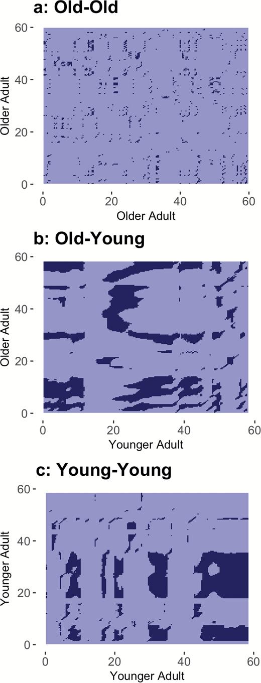
Cross-recurrence plots of head movements for three conversations. The dyads in conversation consist of (a) two older adults, (b) one younger and one older adult, and (c) two older adults.
By sheer examination, it is difficult to tell which of the old-old and young-old conversations show stronger symmetry patterns. To find out, we must move away from qualitative measures and quantify the specific amounts of recurrence in each conversation.
Quantification of Recurrence
Percent recurrence and percent determinism for each of the individuals and for each dyad are shown in Table 1. At least within this sample, it is clear that younger adults showed quite a bit more overall recurrence in their own movements than did older adults, as well as more determinism. However, younger adults also showed increased laminarity, implying more static and stable movements. Further, the embedding dimension of younger adults is higher, implying that the patterning of their movements is more complex. A formal statistical analysis such as a mixed-effects regression predicting differences in percent determinism from actor age across a larger sample of conversations would allow us to test and possibly reject the null hypothesis that younger and older adults show similar amounts of recurrence in conversation. A larger sample would of course be needed to rule out alternative hypotheses, such as gender and personality effects.
Quantitative Characteristics of Individuals: Recurrence Quantification Analysis
| Age group | Optimized embedding dimension | Percent recurrence | Percent determinism | Average line length | Laminarity |
|---|---|---|---|---|---|
| Older | 2 | 8.04 | 71.91 | 3.17 | 70.20 |
| Older | 1 | 3.46 | 22.68 | 6.86 | 11.60 |
| Younger | 6 | 16.66 | 96.23 | 7.74 | 94.70 |
| Younger | 3 | 20.43 | 95.00 | 8.27 | 96.96 |
Note: Older adults’ ages ranged from 69 to 72. Younger adults were 19 years old.
There are large differences among the three conversation classes shown in Figure 5 and these are reflected in the recurrence and determinism percentages in Table 2.
Quantification of Characteristics of Conversation: Cross-Recurrence Quantification Analysis
| Age of partner 1 | Age of partner 2 | Optimized embedding dimension | Percent recurrence | Percent determinism | Longest line length | Average line length |
|---|---|---|---|---|---|---|
| Older | Older | 2 | 3.64 | 43.02 | 6 | 2.3 |
| Older | Younger | 7 | 22.23 | 98.40 | 34 | 8.00 |
| Younger | Younger | 6 | 18.87 | 96.63 | 47 | 8.41 |
Note: Older adults’ ages ranged from 69 to 72. Younger adults were 19 years old.
Our initial prediction that younger and older adults would show more recurrence when talking to others their own age did not seem to be upheld in this data set, as recurrence and determinism are fairly similar in both cases involving younger adults, and are much lower in the old-old case. If anything, there seems to be an increase in both determinism and laminarity in the young-old conversation. With a larger sample, a regression predicting these quantities from actor age and age match (e.g., coded same age group = 1, different age group = 0) might be able to test the null hypotheses that there are no differences between age groups, that there is no “like-me” bias, or test for an interaction between the two processes.
Discussion
Age Differences in Recurrence
The present study illustrated how RQA and CRQA can be applied to time series data to compare the characteristics of a dynamic process, here conversational movements, at different stages across the life span. Our initial results indicate that younger adults may show more repetitive patterning, more stability, and more predictability in their movements in conversation. In conversation with others, younger adults show greater mirroring but less overall change in their head movements. These results further suggest that conversation partners may not be influenced by a “like me” bias. Instead, having two older adults in the conversation seems to qualitatively change the amount and type of patterned and repetitive movements that appear in the conversation.
Older adults show less self-similarity and less determinism in their movements than do younger adults, reflecting less patterned, less repetitive, and less predictable behavior, although this may be driven primarily by periods of limited movement. Conversations between two older adults also show less temporal symmetry (e.g., less “mirroring”) suggesting that older adults may rely less on their coconversants movements, possibly to minimize the cognitive load of integrating their own movements with those of their counterparts. It may also be attributable to physical factors such as muscle tone and energy level. Given the exploratory nature of this work, further study is needed to confirm that these results are systematically age-related and not results of individual differences in personality, topic, or emotional content.
It is important to note that recurrence in velocity of head movements is only one way of quantifying repetition of patterns in conversation and it does not take into account the qualitative meaning of movements, such as the semantic content of deictic gestures. This may lead some combinations of movements, such as head nods and head shakes, to be considered recurrent, even though they are not similar in meaning or sentiment.
RQA and CRQA as a Dynamical Approach
Although we do not present a formal statistical test here, our pilot results imply that a confirmatory test of these hypotheses is warranted. These results also illustrate the benefits of RQA and CRQA measures at capturing the characteristics of dynamic processes at work in aging. From an individual differences approach, these methods take into account intraindividual variability. At the same time, the hyperparameters and outcome measures can be compared across individuals or groups, making it possible to model within-person characteristics in a between-person world. Although they are computationally simple, RQA and CRQA are robust dynamical systems methods, which can quickly and succinctly capture the dynamics of very complicated systems.
As the size and scale of longitudinal data collection expands, it becomes increasingly important to be able to measure the dynamics of intraindividual and intradyad change and to understand how those dynamics differ across groups. The nearly assumption-free nature of RQA and CRQA analyses allow a researcher to find patterns in arbitrarily complex data sets even when little knowledge of the underlying dynamics of the system is available.
Software to perform RQA and CRQA are available both for R (e.g., crqa: Coco & Dale, 2014; tseriesChaos: Di Narzo, 2013), MATLAB (Marwan, 2013; Marwan, Romano, Thiel, & Kurths, 2007), and Python (Rawald, Sips, & Marwan, 2016) and a tutorial walking through the plotting and analysis tools used here is available on the Penn State Quantitative Developmental Systems Group website (http://quantdev.ssri.psu.edu/).
Cautionary Notes
It is important to note that RQA and CRQA are not, in and of themselves, statistical tests, and neither inherently contain a specific hypothesis test nor return a structured p value. Rather, these methods provide a transformation of data sets that can bring to light the underlying dynamics and forces at work in a nonstationary system. Visualization of the recurrence relationship, while useful, is an exploratory and qualitative technique. It is left to the user to interpret the results of these transformations and to apply appropriate statistical tests to examine them.
Further, it is vital to remember that overall recurrence represents only one type of commonality in a dyadic system. Although more detail is visible in the recurrence plot itself, the percentages of recurrence and determinism reported by RQA and CRQA are global measures of repetition which aggregate the recurrence relationships of all time points across both members of the dyad and throughout the entire conversation. In our example, recurrence can be seen between movements that happen at the very beginning of the conversation with those that happen at the very end of the conversation. Other approaches, such as windowed RQA and CRQA, windowed cross-correlation, or DRPs provide local approaches that limit the span of time in which they search for similarity and distinguish one participant’s mirroring actions from the other’s. These approaches may therefore capture different effects that those revealed by the analyses reported here.
Conclusions and Future Directions
Modern data collection tools make it possible to collect intensive time series data about individuals in their day-to-day life and over the course of the process of aging. As these data become increasingly available, we must turn to more dynamical techniques to understand the processes at work and how they evolve and change across time and age. RQA and CRQA stem from a deep and well-traveled approach to dynamical systems modeling. These methods are only the beginning and offer great opportunities to the interested scholar who wishes to model intricate dynamical data sets. As the dynamics of the underlying processes of aging become better understood, these tools and other dynamical systems approaches will allow us to better model, analyze, and predict behavior and change in older, analyze, and predict behavior.
Funding
Research support was provided from the National Institute on Aging (NIA) research grant R21AG041035. This content is solely the responsibility of the authors and does not necessarily reflect the views of the NIA.
Acknowledgments
The authors wish to thank the study participants for taking the time to participate in the experiments included in this study.
References

